The Half-Life of Information

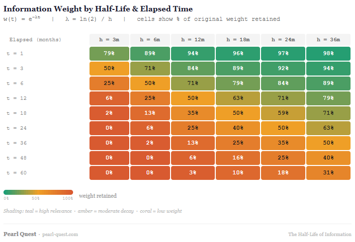
A Practical Tool for Forecasting Systems

In finance and data science, we often assume that more data is better.

But in reality, not all data ages equally.

Some information remains relevant for years. Some becomes obsolete within months.

This is where the concept of half-life becomes powerful.

What Is a Half-Life?

At its core, half-life is a simple idea:

The half-life is the time it takes for the influence of information to decay by 50%.

It comes from physics (radioactive decay), but it translates beautifully into forecasting.

The mathematical form is exponential decay:

w(t) = e^(−λt)

Where:

• w(t) = weight of information at time t
• λ = decay rate
• t = time elapsed

The half-life (h) is directly related to λ, so instead of choosing an abstract decay parameter, you can think in intuitive terms: “How long until this information is only half as useful?”

Why Half-Life Matters in Forecasting

In a rolling-window forecasting system like the one I’ve been developing, the goal is to predict one year ahead using monthly data.

That creates an immediate tension:

• Older data provides sample size and stability
• Recent data provides relevance and signal

A fixed rolling window (e.g., 60 months) treats all observations equally. But markets don’t behave that way.

Information decays.

Half-life allows us to respect that decay without throwing data away.

From Rolling Windows to Weighted Memory

Instead of a hard cutoff (include vs. exclude), half-life gives you a continuous weighting scheme.

This is especially useful when forecasting 12 months ahead, where structural relationships evolve, regimes shift, but long-term patterns still matter.

A Practical Example

Mutual information (mi) scores are one way to select relevant variables. Consider mutual information (mi) smoothing:

mi_dt[, MI_smoothed := mi_alpha * MI + (1 - mi_alpha) * MI_prev]

This is effectively a discrete approximation of exponential decay.

• mi_alpha → controls decay speed
• Equivalent to → choosing a half-life

We can make that explicit. Instead of tuning mi_alpha arbitrarily, define a half-life (h):

α = 1 − e^(−ln(2)/h)

Interpretation:

• Short half-life (e.g., 3 months) → fast adaptation → more responsive, less stable
• Long half-life (e.g., 18 months) → slower decay → more stable, less reactive

Why This Matters for the Forecast Engine

The system is doing several advanced things simultaneously: rolling windows, mutual information feature selection, GAMs with interactions, and monthly data forecasting 12 months ahead.

Half-life thinking improves three critical areas:

A Simple Rule of Thumb

For a 12-month forecast horizon, a half-life of 6–18 months is a strong starting point.

Why? Shorter than the forecast horizon → too reactive. Much longer → too slow to adapt.

The Bigger Insight

Half-life reframes how we think about data:

Data is not just included or excluded. It has memory, and that memory fades over time.

In forecasting systems, this shift is subtle but powerful. It moves you from static datasets to dynamic, time-aware information systems.

Closing Thought

In complex forecasting systems, performance doesn’t just come from better models.

It comes from better treatment of information.

Half-life is one of the simplest, and most powerful, ways to do that.