
A companion to the September 2026 EconPulse brief, which covers the same quarter from the macro side. This note stands on its own and assumes no familiarity with it.
Summary
Through the first three quarters of 2026, the Russell 2000 outperformed the S&P 500 by roughly five percent in each of the first two quarters, then underperformed by nearly ten percent in the third. Read as a single series, that looks like a small-cap cycle: a rally, then a reversal.
It was not. Decomposing the spread against an equal-weighted S&P 500 shows that the two quarters of outperformance came from almost entirely unrelated mechanisms, and that the third quarter reversed only one of them.
Three findings follow from that decomposition.
First, the "small cap versus large cap" spread is not a measurement of one thing. It is the sum of a size effect and a market concentration effect, and those two components can move independently and in opposite directions. In the first quarter of 2026 they did.
Second, the relationship between small caps and interest rates is regime-contingent, and the regime changed twice. Over 2003 to 2021, rising yields were associated with small caps outperforming. The real-yield channel inverted around 2022 and that inversion is robust. The inflation-expectations channel appears to have inverted in 2026, but it is the weaker of the two claims and does not survive a conservative standard-error correction.
Third, the market did not sort on size in the third quarter and it did not sort on profitability. It sorted on growth against value, and that sorting moved with real yields at every point on the size spectrum. The natural reading is a duration effect, and we test it directly. The mechanism passes. The explanation does not: duration was operating everywhere and was decisive only among small caps, because at the top of the market something larger ran the other way.
The note closes with what we could not explain, which is what that larger force was.
Method
All figures use dividend- and split-adjusted daily closes. The equity universe is represented by liquid index funds: IWM for the Russell 2000, SPY for the cap-weighted S&P 500, RSP for the equal-weighted S&P 500, IJR for the S&P SmallCap 600, IJH for the S&P MidCap 400, and IWO and IWN for Russell 2000 growth and value.
The core decomposition is arithmetic rather than a model. Since SPY and RSP hold the same five hundred companies and differ only in weighting, the gap between them isolates the effect of concentration from everything else:
(IWM − SPY)  =  (IWM − RSP)  +  (RSP − SPY)
                 size effect     concentration effect
The size effect compares small caps to the average large-cap company. The concentration effect compares the average large-cap company to the index that contains it. Neither requires an assumption.
Interest rate work uses the ten-year nominal yield decomposed into its two observable components: the ten-year TIPS real yield (FRED series DFII10) and the ten-year breakeven inflation rate (T10YIE). Both begin in 2003, which also marks the inception of RSP, so the full sample runs from May 2003 to September 2026 and contains 5,849 daily observations. The two components correlate at only −0.16 over that period, which is low enough that their coefficients are separately identified.
Every regression is reported with two t-statistics: the ordinary least squares figure and a Newey-West figure corrected for heteroskedasticity and autocorrelation, with Bartlett kernel lag truncation set by the standard automatic rule. The correction changes no coefficient, since it alters only the covariance estimate, so no sign in this note depends on the choice. It changes three t-statistics enough to move them across the 5% threshold, all three downward, and each is flagged where it appears. We report both rather than the flattering one.
Finding one: the spread measured three different things
| Quarter | IWM | RSP | SPY | IWM − SPY | Size | Concentration |
|---|---|---|---|---|---|---|
| Q1 Jan–Mar | +0.92% | +0.61% | −4.47% | +5.39% | +0.31% | +5.08% |
| Q2 Apr–Jun | +19.42% | +10.70% | +14.08% | +5.34% | +8.72% | −3.38% |
| Q3 Jul–Sep | −7.54% | −1.88% | +2.35% | −9.89% | −5.66% | −4.23% |
Cumulative log returns.
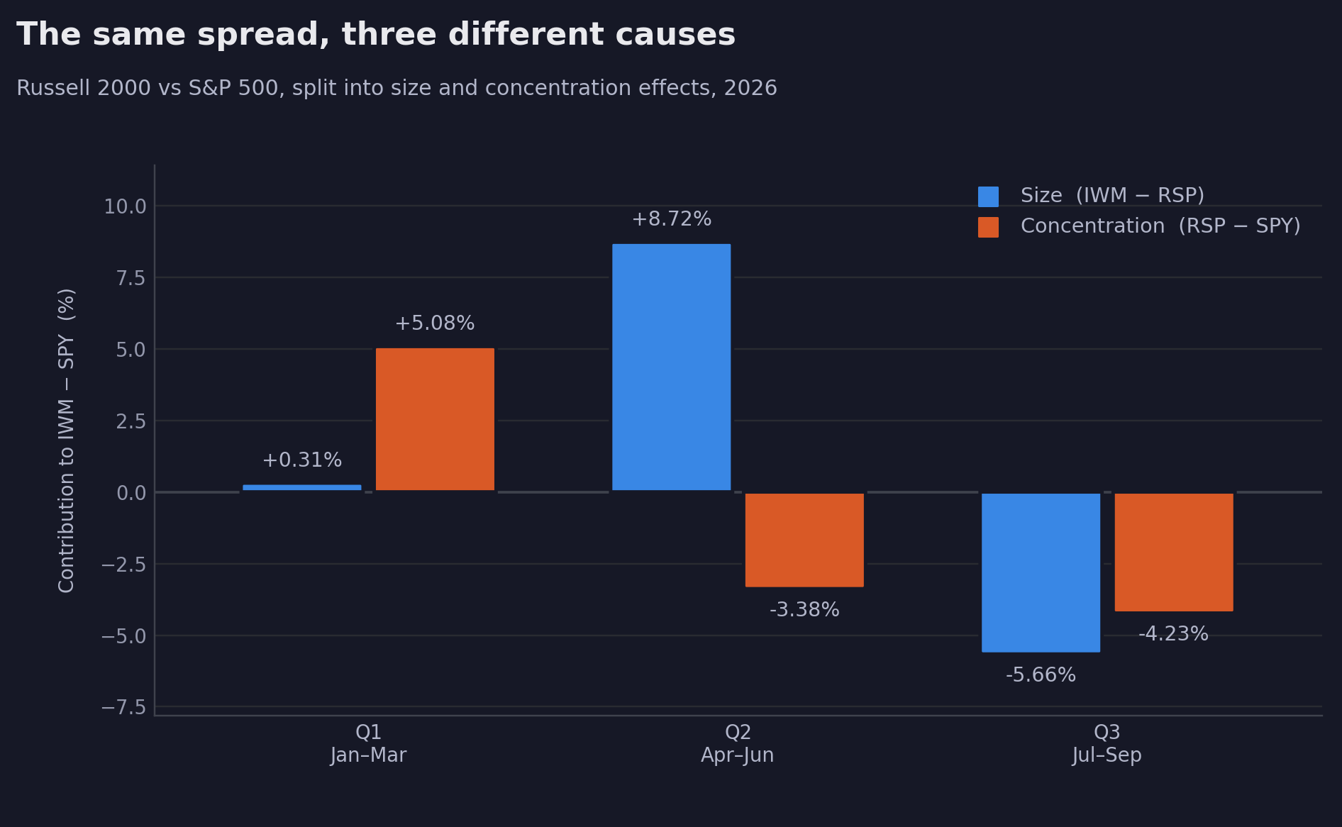
The first two quarters produced nearly identical headline spreads, at +5.39% and +5.34%. The mechanisms behind them have almost nothing in common.
The first quarter was not a small-cap rally. The size effect was +0.31%, which is indistinguishable from zero. The entire spread came from concentration: the cap-weighted index fell 4.47% while the average constituent rose slightly. Small caps did not outperform so much as decline to participate in what was falling.
Constituent attribution confirms it. Using current index weights, the ten largest S&P 500 holdings returned −9.58% in the first quarter while the other 490 returned −1.14%. Microsoft lost 23.3%, Tesla 17.3%, Meta 13.3%. This was a top-ten event, not a market event.
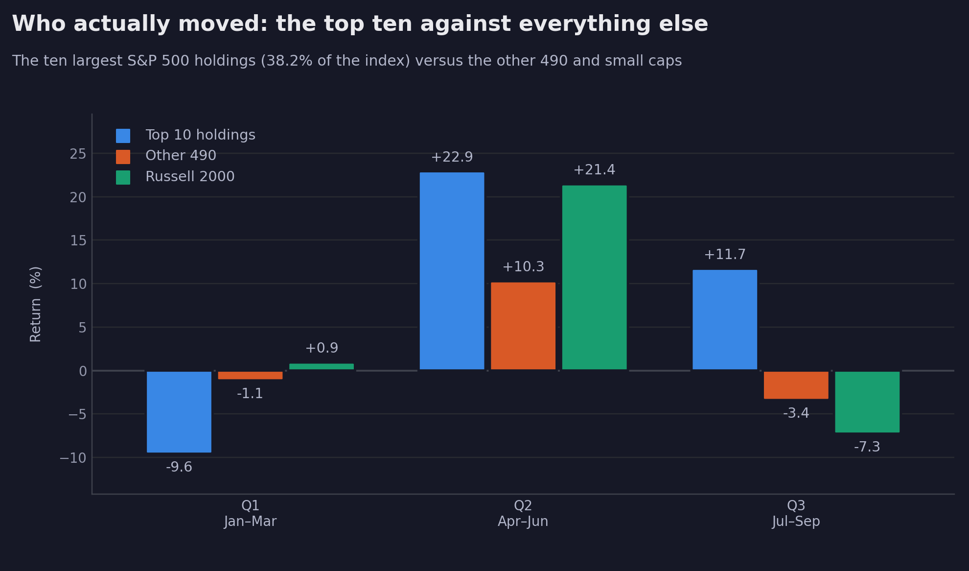
The second quarter was the genuine small-cap episode. The size effect was +8.72%, large and real. Small caps beat the average large-cap company on their own merits, and they did so while concentration ran against them, since the top ten gained 22.94% against 10.28% for the other 490. Everything rose; small caps rose more.
The third quarter inverted the first. The top ten gained 11.72% while the other 490 fell 3.40%, a spread of 15.1 percentage points. Stripped of its ten largest holdings, the S&P 500 would have returned −2.10% rather than +2.38%. (The +2.38% is the full-index figure from the same constituent attribution, which uses September 25 weights; SPY's realized return was +2.35%, and the small gap is the weight drift discussed under Sample constraints.)
The practical consequence is that an investor tracking "small caps versus the S&P" in the first quarter was, without knowing it, tracking a mega-cap drawdown. The same number in the second quarter tracked something else entirely.
Finding two: the rate relationship inverted twice
The conventional claim that small caps are rate-sensitive is true but badly underspecified. The sensitivity has a sign, and the sign depends on which component of the yield is moving.
Regressing the daily size spread on changes in the real yield and the breakeven inflation rate:
| Period | Real yield | Breakeven | R² | n |
|---|---|---|---|---|
| 2003–2021 | +0.0075 (t +4.33 / +2.72) | +0.0127 (t +5.00 / +3.25) | 0.008 | 4,666 |
| 2022–2025 | −0.0092 (t −2.73 / −2.32) | +0.0134 (t +2.20 / +1.76) | 0.014 | 996 |
| 2026 | −0.0393 (t −2.86 / −2.60) | −0.0496 (t −2.05 / −1.81) | 0.070 | 187 |
Coefficients in percent of relative return per basis point. Two t-statistics are shown for each: ordinary least squares first, then Newey-West corrected for heteroskedasticity and autocorrelation. Italicised values fall below the 5% threshold once corrected. Bold marks coefficients significant under both.
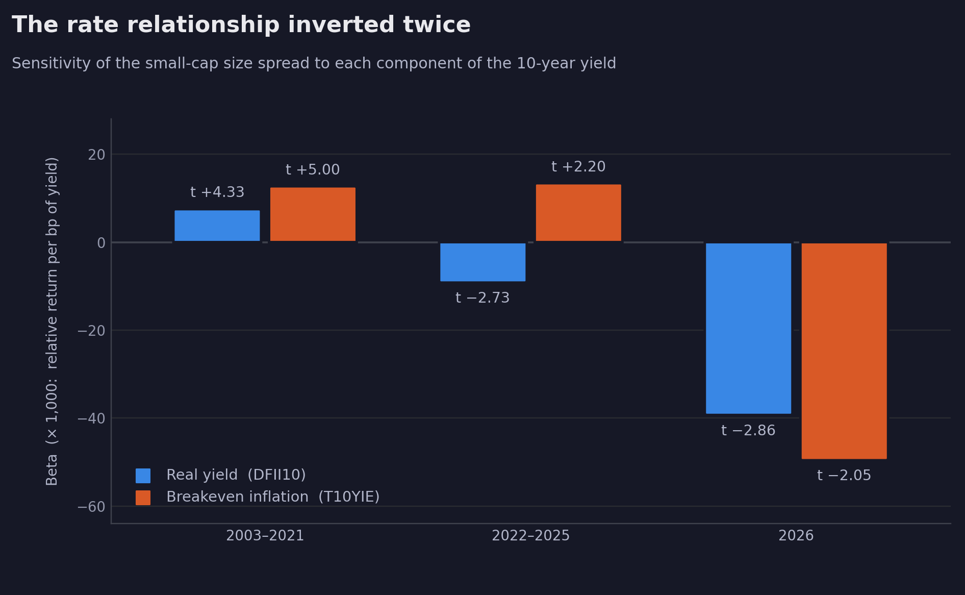
For most of the sample, rising yields of either kind accompanied small-cap outperformance. That is economically sensible. Rising real yields carried growth information, and rising breakevens carried reflation, both of which favor cyclical, domestically exposed, operating-leveraged companies.
The real-yield channel inverted around 2022, when policy rates left zero and financing costs became binding for companies that borrow short and float. Annual betas read −0.0089 in 2022, −0.0113 in 2023, and −0.0410 in 2024, with 2025 a positive exception at +0.0184.
The breakeven channel stayed positive through all of that and turned negative in 2026, which would be the year inflation expectations stopped reading as growth and started reading as a margin threat and a tightening trigger. We state this more tentatively than the real-yield result, and the table shows why. Under ordinary least squares the 2026 breakeven coefficient clears the 5% threshold at t −2.05. Correct the standard errors for autocorrelation and it falls to −1.81, which clears 10% but not 5%. The point estimate does not move, and it is the largest in the sample by a wide margin, but we are not going to call a result significant on the strength of the less conservative of two standard errors.
So 2026 is the only year in twenty-three where both components are negative, and the real-yield leg of that is solid while the breakeven leg is suggestive. On the full-sample nominal relationship, 2026's beta of −0.0423 sits 3.06 standard deviations below the twenty-four year annual mean of +0.0068, and is the most negative in the sample. On the scale-free correlation measure, which cannot be inflated by a small denominator, 2026 ranks first of twenty-three at −0.264 against a mean of +0.060. Yield volatility in 2026 was unremarkable, at roughly the 30th percentile of annual values, so this is not an artifact of a quiet denominator.
The level context matters as much as the changes. The ten-year real yield now stands at 2.93%, the 99.7th percentile of its history since 2003, against a 2003–2021 average of 0.84%. Breakevens at 2.36% sit at only the 73rd percentile. Whatever is happening is more a real-rate phenomenon than an inflation-expectations phenomenon, notwithstanding that both channels turned.
Finding three: duration was present everywhere and decisive only at the bottom
If the third quarter were about size, the damage should scale with size. If it were about balance-sheet fragility, a profitability screen should matter. Neither holds.
| Segment | Q3 2026 |
|---|---|
| SPY, cap-weighted S&P 500 | +2.35% |
| RSP, equal-weighted S&P 500 | −1.88% |
| IWN, Russell 2000 Value | −5.05% |
| IJH, S&P MidCap 400 | −6.62% |
| IWM, Russell 2000 | −7.54% |
| IJR, S&P SmallCap 600 | −8.27% |
| IWO, Russell 2000 Growth | −9.77% |
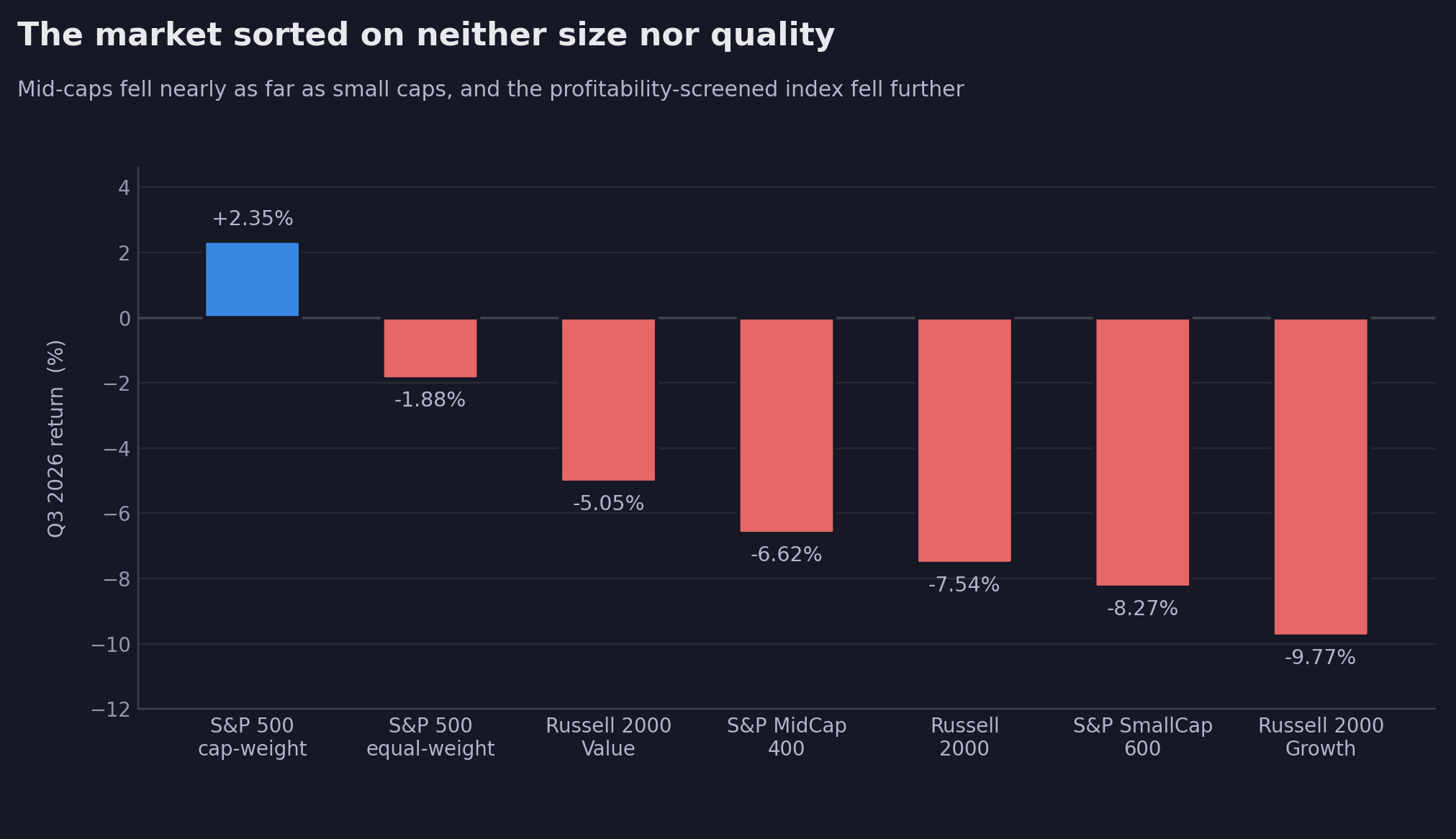
The quality screen fails. The S&P SmallCap 600 requires positive earnings; the Russell 2000 does not. If unprofitable companies were the mechanism, the Russell should have fallen further. It fell less, at −7.54% against −8.27%. Profitability is not what sorted this market.
The size gradient is weak. Mid-caps fell 6.62%, nearly as far as small caps at 7.54%. The gap from mid-cap to large is −4.73% against −5.66% for small-cap to large, so most of the damage occurs moving from mega-cap to everything else, not from mid-cap down to small.
What is left is growth against value. Small growth underperformed small value by 4.71% in the quarter. That is the one sorting variable still standing, and it invites the duration explanation, so we tested it rather than asserting it.
Testing duration directly
Equity duration is the same idea as bond duration applied to a cash flow stream nobody has promised you. A bond's price is the present value of a known schedule, and duration is the weighted average time until the money arrives, which is what determines how far the price moves when the discount rate moves. A stock is also a present value, except the schedule is a forecast. A company earning its money now behaves like a short bond. A company whose valuation rests on profits expected in 2035 behaves like a long one, because discounting compounds over time.
Under a constant-growth dividend discount model, equity duration works out to approximately (1+r)/(r−g) while the price-earnings multiple is approximately 1/(r−g). Duration is therefore roughly proportional to the multiple, which makes growth the long-duration leg and gives us something measurable. We did not have to build the sort ourselves: S&P and FTSE Russell construct their growth and value indices from constituent valuation multiples, so the growth-minus-value spread is the multiple sort, done with full constituent data we do not possess.
If the third quarter was a duration repricing, the prediction is unambiguous. Growth should have lost to value in every size bucket, and lost most where duration is longest, which is large-cap growth.
| Growth minus value, Q3 2026 | Real-yield beta, 2026 | Predicted by the rate move | Realized | Residual |
|---|---|---|---|---|
| Russell 1000 (large) | −0.0482 (t −2.49 / −2.95) | −2.96% | −1.65% | +1.31 |
| S&P 500 (large) | −0.0654 (t −3.34 / −3.94) | −4.16% | +2.54% | +6.70 |
| S&P MidCap 400 | −0.0314 (t −2.26 / −2.14) | −2.46% | −0.16% | +2.30 |
| S&P SmallCap 600 | −0.0287 (t −2.80 / −2.53) | −2.40% | −4.51% | −2.11 |
Predicted applies each spread's own 2026 daily betas to the quarter's actual move in the real yield and the breakeven, which were +68 and +13 basis points. Both t-statistics are shown, ordinary least squares then Newey-West. All four clear the 5% threshold under either, and the two large-cap estimates strengthen under correction.
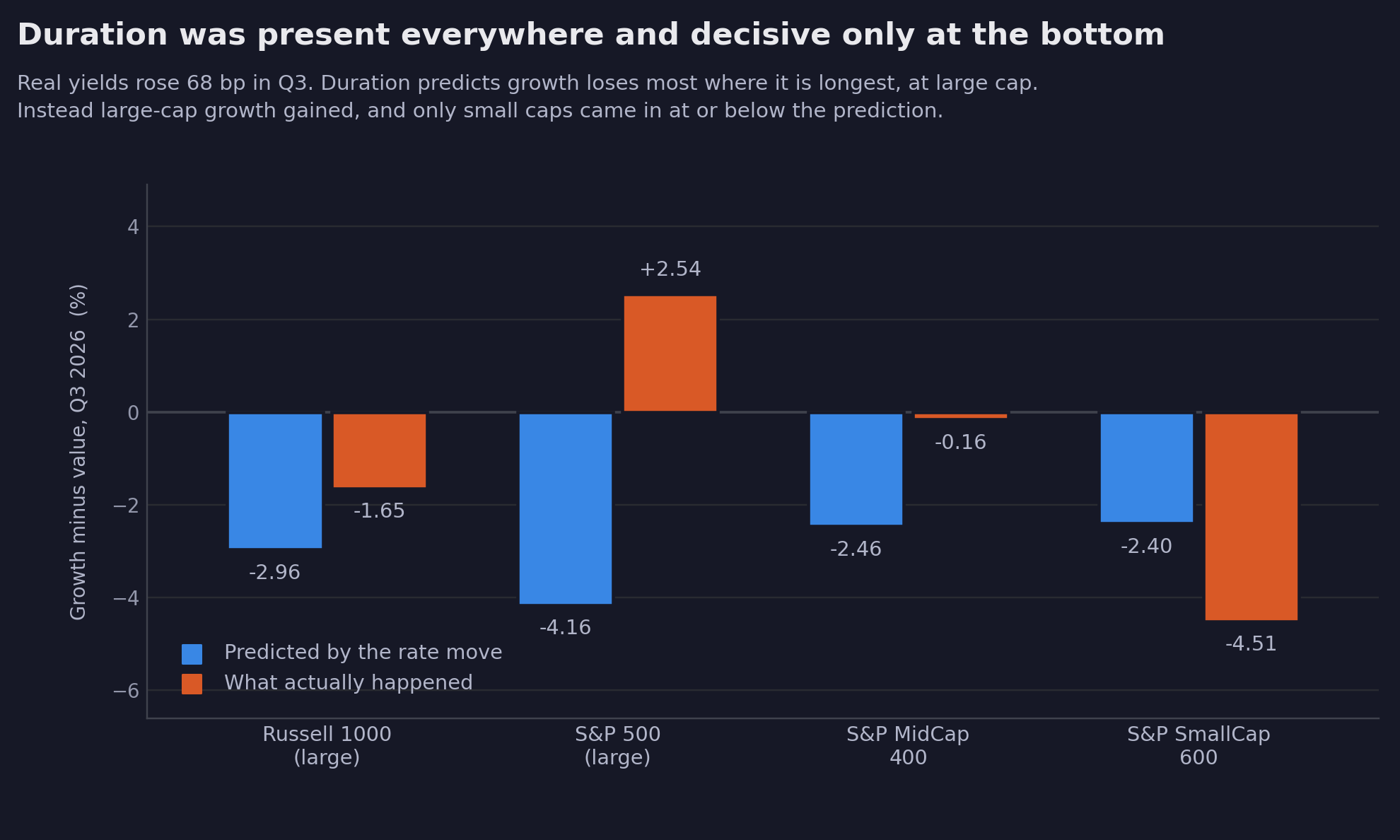
The mechanism passes. Every one of the four spreads carries a significantly negative real-yield beta in 2026, and the largest sensitivity sits where duration is longest, in large-cap growth. Over 2023 to 2025 all four were significantly positive: +0.0195, +0.0196, +0.0125 and +0.0159, with t-statistics from +2.64 to +4.66. The inversion documented in Finding two is not a small-cap curiosity. It happened across the entire market, and we can now show it four independent ways rather than one.
This is the most robust result in the note. All eight of those real-yield estimates, four in 2026 and four before it, survive the Newey-West correction that costs the breakeven channel its significance, and the two large-cap estimates get stronger under it rather than weaker.
The explanation fails. Real yields rose 68 basis points, so the duration drag on large-cap growth should have been the worst of the four at roughly −4.2%. Large-cap growth instead beat value by 2.5 points. Only in small caps did the realized spread come in below what the rate move predicts.
Both things are true at once, and reconciling them is the finding. Duration was a real force acting on every segment in the same direction. At large cap it was overwhelmed by something close to seven points larger running the opposite way. At small cap nothing offset it, so it showed up in the realized return. The ordering in the segment table is what a uniform duration drag looks like once you subtract an idiosyncratic shock concentrated at the very top of the index.
That also reframes the open question this note ends on, which is what that offsetting force at the top of the index actually was.
The macro backdrop
Three external developments frame the third quarter, and all three run through the same channel.
The Federal Reserve raised rates on September 16, by 25 basis points to a target range of 3.75% to 4.00%, unanimously. Chair Warsh said "the plain fact is that inflation is too high and has been for too long," and twelve of eighteen Committee participants projected a further increase before year-end. This was the first increase of the cycle.
Energy prices are the transmission mechanism. Brent crude futures settled at $97.82 and WTI at $90.27 on September 30, up roughly 50% and 46% year over year. The path through 2026 has been violent: Brent averaged $70.89 in February, spiked to a monthly average of $117.29 in April, retreated to roughly $84 through June and July as the immediate conflict premium drained, then climbed again to $91.08 in August and higher since. Middle East export flows have recovered to approximately 98% of pre-war levels, but the market remains characterized as undersupplied.
That flows directly into the inflation data. The August CPI report showed headline inflation of 3.4% and core at 2.4%, the best core reading of the cycle. Energy prices rose 16.3% year over year and gasoline 27.4%, with gasoline alone accounting for more than a third of the monthly increase in the all-items index. The aggregate improved while the component households purchase weekly did not.
This is the plausible mechanism behind the breakeven channel inverting. When inflation expectations are driven by an energy supply shock rather than by demand, they stop carrying growth information. A reflationary breakeven helps cyclical small caps. A cost-shock breakeven threatens their margins and invites the tightening that raises their discount rate. Same series, opposite content.
We note this as the most coherent available explanation rather than a tested result. Distinguishing supply-driven from demand-driven inflation expectations rigorously would require decomposition work beyond this note's scope.
What we could not explain
Three limitations, stated plainly.
Why those four companies. The third-quarter concentration effect is not "mega-caps rose" and it is not "the AI trade rose." Five of the top ten holdings fell: Tesla by 15.6%, Micron by 7.7%, Broadcom by 6.9%, and both Alphabet share classes. The entire +4.48 point index contribution comes from four names. Microsoft, Apple, Nvidia and Meta contribute +5.04 points between them, while the other six subtract 0.56. Broadcom and Micron are squarely in the AI complex and both declined, which rules out the thematic explanation.
Finding three sharpens this rather than answering it. Those four were not exempt from the quarter's duration drag. They carried it and beat it, which means the question is not why they escaped a headwind but what delivered a tailwind on the order of seven percentage points to large-cap growth in a quarter when real yields rose 68 basis points. The candidate explanations are passive flows mechanically favoring the largest index weights, active crowding into a narrow group, and company-specific earnings news. Distinguishing between them requires fund flow and positioning data that neither of our data sources carries, and we are not going to guess between three plausible stories in print.
Magnitude beyond regime. Using the stock-bond correlation as a regime proxy and fitting on 2004 through 2025, 2026's regime predicts a size beta of −0.0009. The actual is −0.0423, a residual of 3.55 standard deviations. The regime framework explains the sign of the inversion. It does not explain how large the inversion is.
Sample constraints. The constituent attribution uses index weights as of September 25 applied to a quarter ending September 30, so look-ahead bias is roughly five days of drift and immaterial here. The same method would not survive being pushed into earlier years without point-in-time weights. More broadly, 2026 is one year. The regime claim rests on a single observation of the second inversion, and we would not assert it as a stable property until it persists or recurs.
Implications
For anyone using small-cap exposure as a portfolio sleeve, the operative finding is that the benchmark spread is not diagnostic. In the first quarter of 2026, an investor watching the Russell against the S&P would have concluded that small caps were working. They were not. Mega-caps were failing, and the spread reported that as a small-cap success.
A breadth measure fixes this cheaply. The equal-weight to cap-weight ratio requires two daily series and no constituent data, and it separates the two components that the headline spread conflates. It is a proxy rather than a true participation count, and that distinction should be stated wherever it is presented, but it would have flagged the first quarter correctly in real time.
For the rate relationship, the practical implication is that a stable beta assumption is wrong. The sign has inverted twice in twenty-three years, most recently this year, and the inversions correspond to identifiable macro conditions rather than to drift. Any model that treats small-cap rate sensitivity as a fixed parameter will be correctly signed for long stretches and badly wrong at exactly the turning points that matter.
Data sources: Alpha Vantage (adjusted daily prices, index constituent weights), Federal Reserve Economic Data (DFII10, T10YIE, Treasury constant maturity yields), U.S. Bureau of Labor Statistics (CPI), Federal Reserve (FOMC materials). Micron's +241.7% second-quarter return was verified against raw and adjusted closes with no splits in the window, and reflects the high-bandwidth memory demand cycle.
This note is for educational and informational purposes and does not constitute investment advice. Past performance does not indicate future results.
Replication
Every number in this note can be recomputed from the data behind it. The accompanying archive contains the daily price and yield series as CSV files and a script, verify.py, that reproduces each published figure and prints PASS or FAIL against it. Running it requires only pandas, numpy and statsmodels. It checks 90 figures, including both the ordinary and the Newey-West t-statistics.
Download the replication archive (zip, 1.9 MB)
The script found a genuine error during preparation. An early version computed quarterly returns from the first closing price inside each quarter rather than from the prior quarter's close, which silently discarded the first trading day and moved several figures by up to a full percentage point. The published figures use the prior close. We mention it because a verification step that never catches anything is not a verification step.
What the script cannot check is whether Alpha Vantage's adjusted closes and the Federal Reserve's published yields are themselves correct, the macro narrative drawn from FOMC, EIA and BLS releases, and the interpretation. Numbers constrain a story. They do not write it.
Appendix: supplementary results
Full-sample nominal relationship. Regressing the daily size spread on ten-year nominal yield changes over 2003 to 2026 gives a beta of +0.0049 (t +3.55) with an R² of 0.002. The relationship is positive and economically negligible across the full sample. The annual beta is negative in 7 of 24 years and significantly negative in exactly one.
Rolling estimation. Rolling 126-day betas across 5,723 windows have a mean of +0.0079, are negative in 26.9% of windows, and are significantly negative in 6.3%. The window ending September 29, 2026 reads −0.0682 (t −5.26), the 0.1st percentile. The most negative window in the sample ends September 2, 2026.
Regime split by stock-bond correlation. Splitting the full sample by the sign of the 126-day correlation between equity returns and yield changes: in the growth regime, which covers 76% of days, the size beta is +0.0076 (t +4.87, or +3.13 Newey-West corrected); in the inflation and policy regime, 24% of days, it is −0.0077 (t −2.52, falling to −1.96 corrected, which sits exactly on the threshold and should be read as suggestive rather than established). Across years, a year's mean stock-bond correlation correlates +0.51 with its size beta (t +2.73, R² 0.26). The current reading of −0.549 sits at the 0.2nd percentile of twenty-three years.
Episode frequency. Measured against all rolling 63-day windows since 2003, the third quarter of 2026 sits at the 5.7th percentile for the size component and the 7.4th for the concentration component. Roughly a one-in-seventeen quarter for each. Unusual, but not without precedent, and frequent enough that a breadth indicator would signal periodically rather than only in crises.
Concentration-leg rate sensitivity. The concentration spread shows a strongly positive rate relationship over 2003 to 2021 (real t +7.45, breakeven t +10.68) which turns negative over 2022 to 2025. In 2026 the real-yield channel is insignificant (t +1.18) while the breakeven channel is negative (−0.0361, t −1.96). Rates explain very little of the concentration effect in the current period, which is consistent with it being driven by something other than discount rates.